Introduction
Pivot Table is one of the killer features of Microsoft Excel. It is a quick and easy way to analyze Excel data in summary form, by creating various views, in a few short steps.
This article walks you through on how to make a Pivot Table in Excel.
For this illustration, let us use the Sales By Product By Party Sheet generated from ERP One.
A sample XL sheet is shown below.
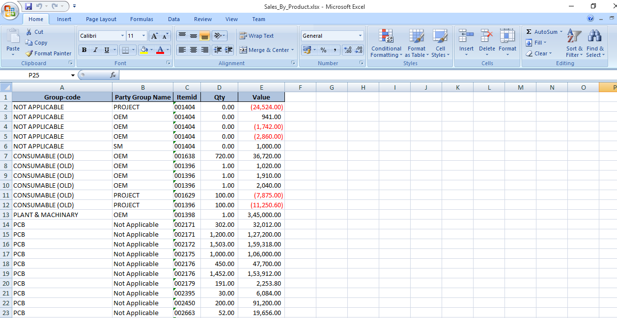 We have kept only five relevant columns and removed the rest to keep this illustration simple.
Inserting Pivot Table
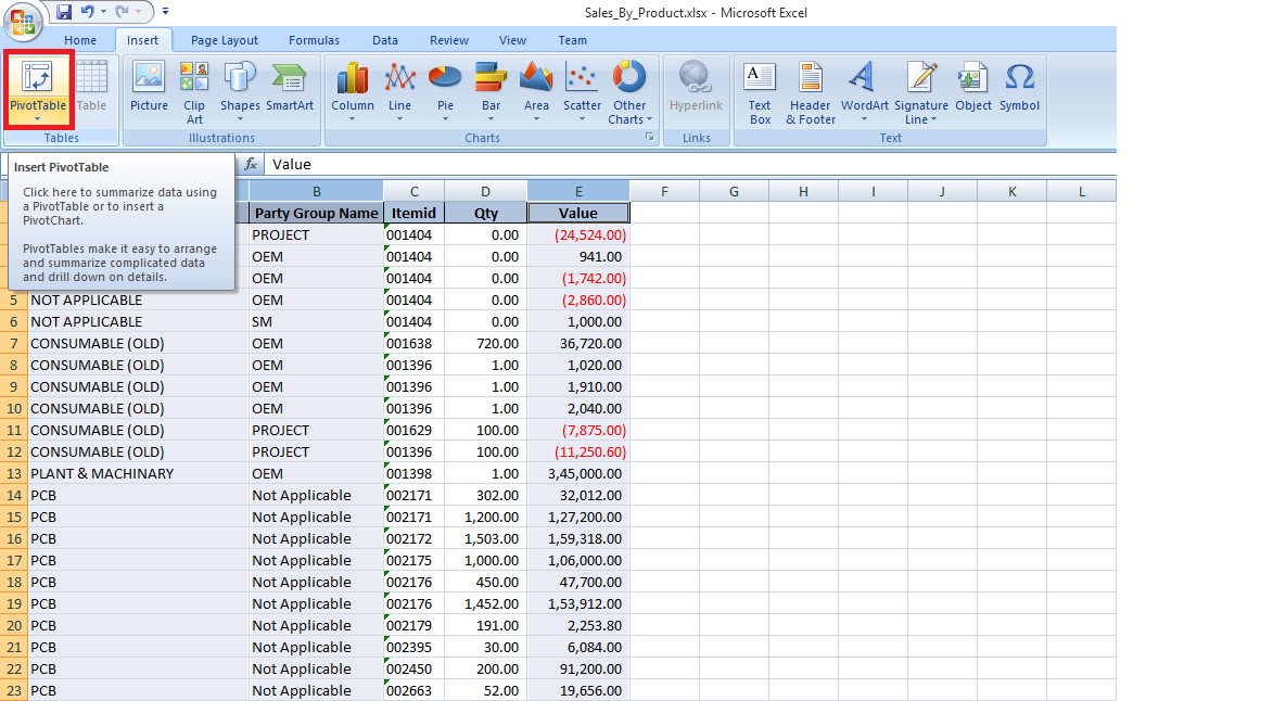
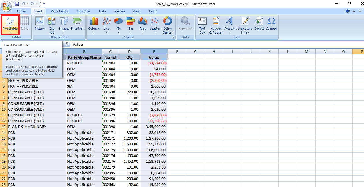
First select and highlight the range of cells which would form part of the data to be analyzed.
From the Menu, select [Insert]>>[Pivot Table].
Specify Pivot Table options
Data range is prompted by Excel as per the range selected by you.
You can also choose where to insert the new Pivot table.
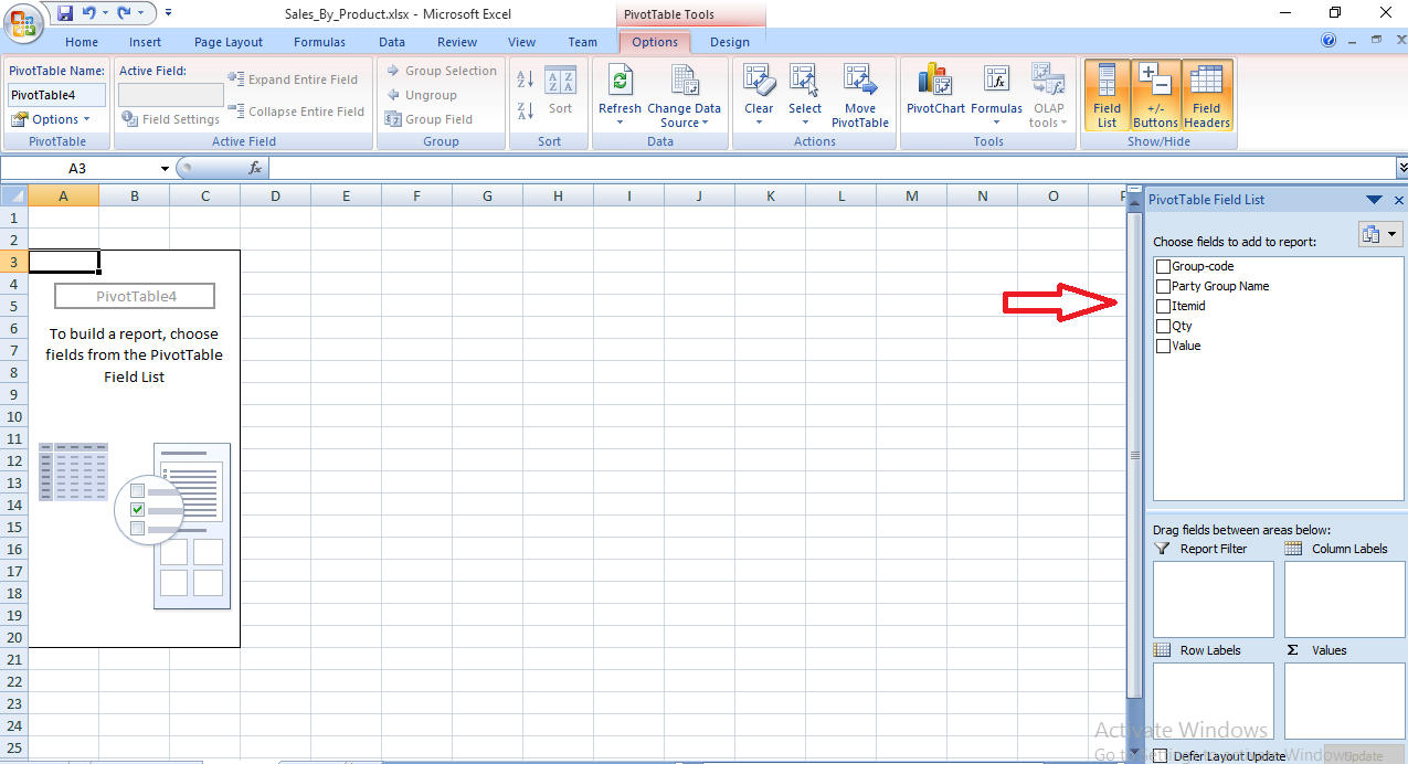
Pivot Table selection
To the right of your Excel Sheet, you can see the fields to be selected.
On the bottom part, you can select and arrange the fields through drag-n-drop.
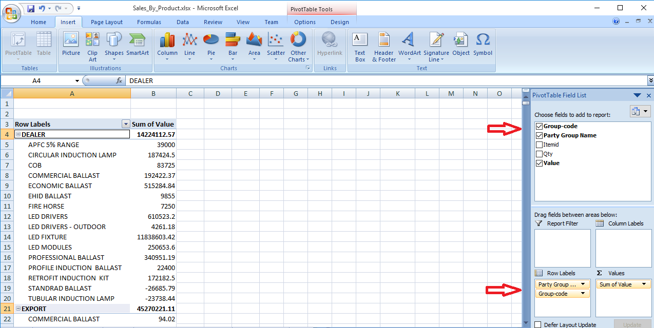
Select the columns
In the snapshot, we have selected 3 columns.
The fields get arranged in the bottom portion, in the order in which you click. You can rearrange them, if you want.
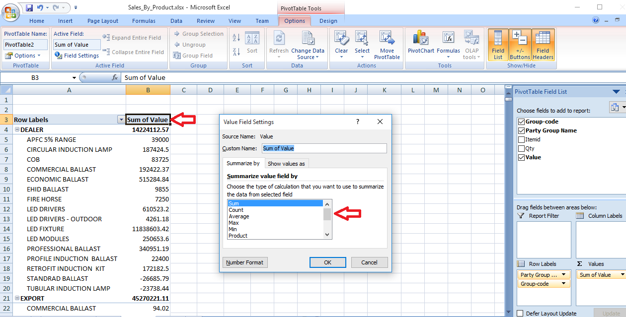
Summarize Value Field
You can select how to summarize your result - whether to count or sum, average etc.
We have selected [Sum] for this illustration.
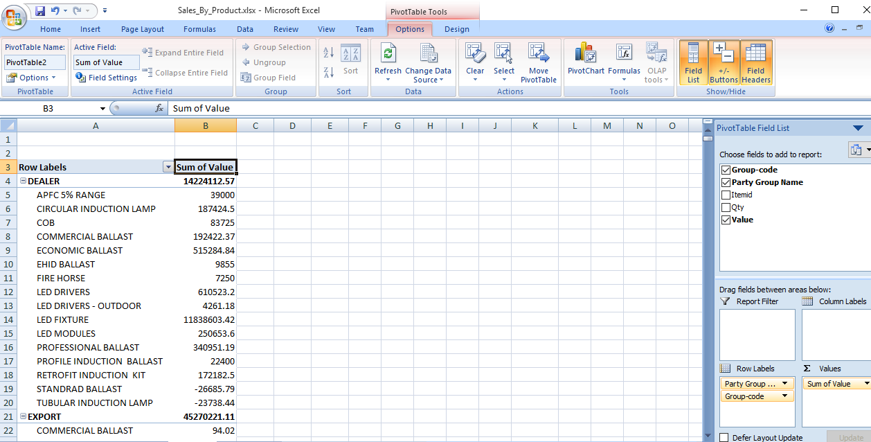
Pivot table
Your Pivot table is now created, showing sales value of every [Party Group] over various [Item Group].
If you just drag-n-drop [Group Code] above [Party Group] in the right bottom portion, your Pivot table will change to show sales of Item groups over Party Group.